library(dplyr)
library(tidyr)
library(ggplot2)

set.seed(42)

n_sims <- 500
n_years <- 3

harvest_scenarios <- c(low = 0.1, high = 0.3)

sigma_obs <- 15 # initial-condition sd, same value reused as observation-error sd
mu_r <- 0.4 # mean of the growth-rate parameter distribution
sigma_r_param <- 0.08 # parameter uncertainty in the mean growth rate
sigma_r_process <- 0.1 # process uncertainty: year-to-year noise around the drawn mean
K <- 500 # carrying capacity, used only by the logistic growth function

growth_exponential <- function(N, r) N * exp(r)
growth_logistic <- function(N, r) N + r * N * (1 - N / K)
growth_functions <- list(
    exponential = growth_exponential,
    logistic = growth_logistic
)

simulate_trajectory <- function(growth_fun, h) {
    N_true <- numeric(n_years + 1)
    N_true[1] <- rnorm(1, mean = 200, sd = sigma_obs) # initial-condition uncertainty
    r_mean <- rnorm(1, mean = mu_r, sd = sigma_r_param) # parameter uncertainty

    for (t in seq_len(n_years)) {
        r_t <- rnorm(1, mean = r_mean, sd = sigma_r_process) # process uncertainty
        N_grown <- growth_fun(N_true[t], r_t) # structural uncertainty (which growth_fun)
        N_true[t + 1] <- max(N_grown * (1 - h), 0) # scenario uncertainty (which h)
    }

    N_obs <- pmax(N_true + rnorm(n_years + 1, mean = 0, sd = sigma_obs), 0) # observation error

    tibble(time = 0:n_years, N_true = N_true, N_obs = N_obs)
}

sims <- expand_grid(
    sim = 1:n_sims,
    structure = names(growth_functions),
    scenario = names(harvest_scenarios)
) |>
    rowwise() |>
    mutate(
        traj = list(simulate_trajectory(
            growth_functions[[structure]],
            harvest_scenarios[[scenario]]
        ))
    ) |>
    unnest(traj) |>
ungroup()6 The different types of uncertainty
“How uncertain am I?” is not one question but several. Asking which kind of uncertainty you’re dealing with is helpful, because they behave differently and some can be reduced while others cannot.
Uncertainty is a scientific concept and we need to be careful when using it outside of scientific settings, such as in science communication. For the general public uncertainty means “we don’t know anything”. For scientists it can mean the same thing, but more commonly it means “we aren’t sure but we can estimate how unsure we are”. Typical examples are confidence and credible intervals, which put a bound on our uncertainty.
Stochasticity is the technical term for this randomness: a process is stochastic if it can’t be predicted exactly, only described in terms of probabilities of different outcomes. A purely random process is essentially unpredictable.
Stochasticity contrasts with a deterministic process, which always produces the same output from the same starting conditions. In ecological models, stochasticity is usually simulated by drawing random numbers from a probability distribution (e.g. adding random draws from a normal distribution to a population growth rate, or drawing survival events from a binomial distribution) and is the reason two runs of the same stochastic model, from the same starting point, can give different trajectories.
Some of the different types of uncertainty we encounter that you might want to model:
- Process (or environmental) uncertainty: genuine randomness in the system itself. The world is stochastic: two identical populations in identical conditions won’t follow identical trajectories. This is irreducible (more data tells you about it but never removes it), and it’s what a process-error term in a dynamic model represents.
- Observation (or measurement) error: the gap between the true state and what you managed to measure. Your survey miscounts; your instrument is noisy. This is a property of the observing, not the system, and it can often be reduced with better methods or more sampling. Keeping process and observation error apart is one of the central problems of state-space modelling, and confounding the two is a classic trap.
- Parameter uncertainty: you’ve settled on a model structure, but you don’t know its parameters exactly; you have estimates with intervals. This is reducible: more (and more informative) data tightens it. This is also the uncertainty that estimation problems such as identifiability and confounding can inflate without you noticing.
- Structural (or model) uncertainty: you’re not even sure the model itself is right, meaning which processes to include, which functional forms, which interactions. This is usually the largest and most neglected source, because it doesn’t show up inside any single model: a model is supremely confident about a world that may not be ours. It’s addressed by comparing models, model averaging, or ensembles, not by collecting more data under one structure.
- Initial-condition and boundary uncertainty: for a dynamic model, uncertainty about where the system starts (or about the forcing pushed in at its edges) that then propagates forward. This is why forecasts can fan out even when the model and parameters are perfect.
- Scenario uncertainty: uncertainty about the inputs you can’t predict at all, such as future policy, harvest, or climate forcing. You don’t normally put a probability on these; you explore them as scenarios (exactly the scenario modelling from earlier).
Reducible uncertainties (observation error, parameter uncertainty) can be shrunk by better data or better measurement, so they’re where “go and measure this” advice pays off.
Structural uncertainties can also be reduced, but usually by doing different types of science, not more of the same. An example would be designing a new type of experiment to test between two competing mechanisms.
Irreducible ones (process uncertainty) have to be represented if we want well-calibrated probability intervals. That means, if we say our interval is a 95% predictive interval, then 95% of predicted events should fall in that interval.
A model that reports tight intervals has usually only accounted for parameter uncertainty and is silently ignoring the rest. That gives a tidy-looking answer more confident than the world warrants.
The uncertainty topic is a minefield with a large literature (and a fair amount of inconsistent terminology), so treat the above as an orientation rather than the last word.
Uncertainty goes beyond your model. The list above is framed around the model and its data, but in applied and management settings the most important uncertainties often in the human system it’s embedded in. Peterman’s (2004) account of fisheries is a concrete example. He identifies five sources of uncertainty in a fishery system, only the first two of which are the “modelling” kinds we’ve discussed:
- Natural variability across space and time in the distribution, abundance, and productivity of the fish populations (our process uncertainty).
- Observation error: imperfect information arising from both measurement error and sampling error.
- Communication difficulties among scientists, managers, and stakeholders about technical scientific information and its associated uncertainties. Sometimes also called linguistic uncertainty, to differentiate it from the epistemic uncertainties we discussed above (Regan, Colyvan, and Burgman 2002)
- Unclear management objectives.
- Implementation error: the gap between a management goal and the actual realised outcome (e.g. the spawning-stock biomass or fishing-mortality rate that actually results).
If your work is meant to inform a decision, sources (3), (4), and (5) can dominate the outcome. That’s why good modellers go beyond modelling and learn to communicate well. Developing your understanding of the problem and building your strength in communication skills are key.
6.1 A worked example: harvesting a population over three years
Let’s look at the six modelling sources of uncertainty above in a small model. Below is a population of a harvested species followed over three annual timesteps, written first as equations and then as an R simulation. We run multiple simulations of the population growth, so we can explore initial condition, observation and process uncertainties that vary within a simulation, as well as parameter, scenario and structural uncertainties that are constant with a simulation but vary across simulations.
6.1.1 The model
Let \(N_t\) be the true abundance of the population at the start of year \(t\), for \(t = 0, 1, 2, 3\). Growth happens first each year, then a fixed fraction of the grown population is harvested. We don’t observe \(N_t\) directly; instead we observe \(Y_t\), a noisy survey estimate of it.
Initial condition. The starting abundance is not known exactly, so it’s a random variable rather than a fixed number: \[ N_0 \sim \text{Normal}(\mu_{N_0} = 200, \ \sigma_{obs} = 15), \qquad N_0 > 0 \] where \(\sigma_{obs}\) is a standard deviation. This is initial-condition uncertainty, and we reuse the same \(\sigma_{obs}\) for observation error below, since both describe how far a single survey estimate typically sits from the true count.
Parameter uncertainty. The mean growth rate isn’t known exactly either. Each simulation run draws its own value of it from a distribution before the population is projected forward: \[ \bar r \sim \text{Normal}(\mu_r = 0.4, \ \sigma_r = 0.08) \] \(\bar r\) is fixed for the whole run once drawn, but it varies between runs, which is what lets us see how much parameter uncertainty alone contributes to the spread of outcomes.
Process uncertainty. Within a run, the realised growth rate still fluctuates year to year around \(\bar r\), because the environment the population experiences is itself stochastic: \[ r_t \sim \text{Normal}(\bar r, \ \sigma_p = 0.1) \] This is irreducible: even if we knew \(\bar r\) exactly, \(r_t\) would still bounce around it.
Structural uncertainty. We’re not sure which growth function is the right one, so we run the whole simulation twice, once under each candidate: \[ N^{grown}_t = \begin{cases} N_{t-1} \, e^{\, r_t} & \text{exponential growth} \\[4pt] N_{t-1} + r_t N_{t-1} \left(1 - \dfrac{N_{t-1}}{K}\right) & \text{logistic growth, } K = 500 \end{cases} \] Both functions use the same drawn \(r_t\), so any difference between them is attributable to structure, not to which random numbers happened to come up.
Scenario uncertainty. After growth, a fixed fraction \(h\) of the population is harvested. We don’t put a probability on \(h\): instead we carry two policy scenarios through in parallel, low harvest and high harvest, \[ N_t = N^{grown}_t (1 - h), \qquad h \in \{0.1, \ 0.3\} \]
Observation error. Finally, the survey that monitors this population doesn’t count \(N_t\) perfectly: \[ Y_t = N_t + \varepsilon_t, \qquad \varepsilon_t \sim \text{Normal}(0, \ \sigma_{obs} = 15) \]
Put together, one simulated trajectory is generated by: draw \(N_0\) and \(\bar r\) once; then for \(t = 1, 2, 3\), draw \(r_t\), apply one of the two growth functions, apply one of the two harvest rates, and add observation noise to get \(Y_t\).
6.1.2 Simulating it in R
Every draw of rnorm() above corresponds to one line of the equations: N_true[1] to \(N_0\), r_mean to \(\bar r\), r_t to \(r_t\), and the final rnorm() on N_true to \(\varepsilon_t\). The structure and scenario columns instead come from which function or harvest rate we chose, not from a random draw, which is exactly the distinction between the reducible/irreducible uncertainties above and the structural/scenario ones.
ggplot(
    sims,
    aes(
        time,
        N_true,
        group = interaction(sim, structure, scenario),
        colour = structure
    )
) +
    geom_line(alpha = 0.05) +
    facet_wrap(
        ~scenario,
        labeller = labeller(
            scenario = c(
                low = "Low harvest (h = 0.1)",
                high = "High harvest (h = 0.3)"
            )
        )
    ) +
    labs(x = "Year", y = "True abundance", colour = "Growth model") +
    theme_minimal()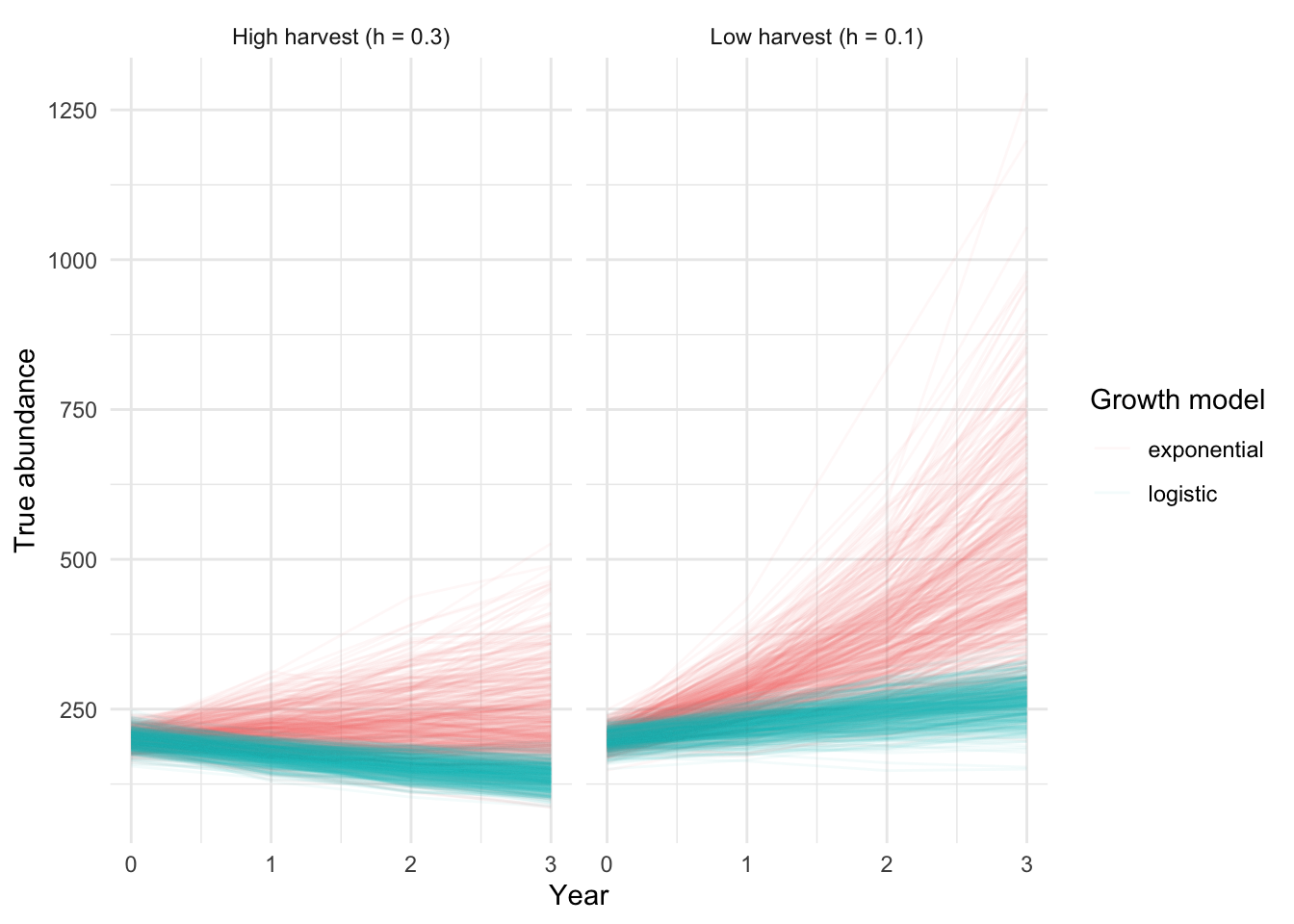
The two model structures diverge (red vs blue lines) because the logistic growth is slowed by density dependence, whereas the exponential growth is unlimited. By year 3 the structural difference dwarfs the spread caused by any other source of randomness.
Its also clear that we get higher numbers after three years with the lower harvest rate.
The last thing to show is how process and observation uncertainty are different. Here is a single simulated run, with the true trajectory (blue) and what the survey actually recorded (red):
one_run <- sims |> filter(sim == 1, structure == "logistic", scenario == "low")

ggplot(one_run, aes(time)) +
    geom_line(aes(y = N_true, colour = "True abundance")) +
    geom_point(aes(y = N_obs, colour = "Survey estimate")) +
    geom_line(aes(y = N_obs, colour = "Survey estimate"), linetype = "dashed") +
    labs(x = "Year", y = "Abundance", colour = NULL) +
    theme_minimal()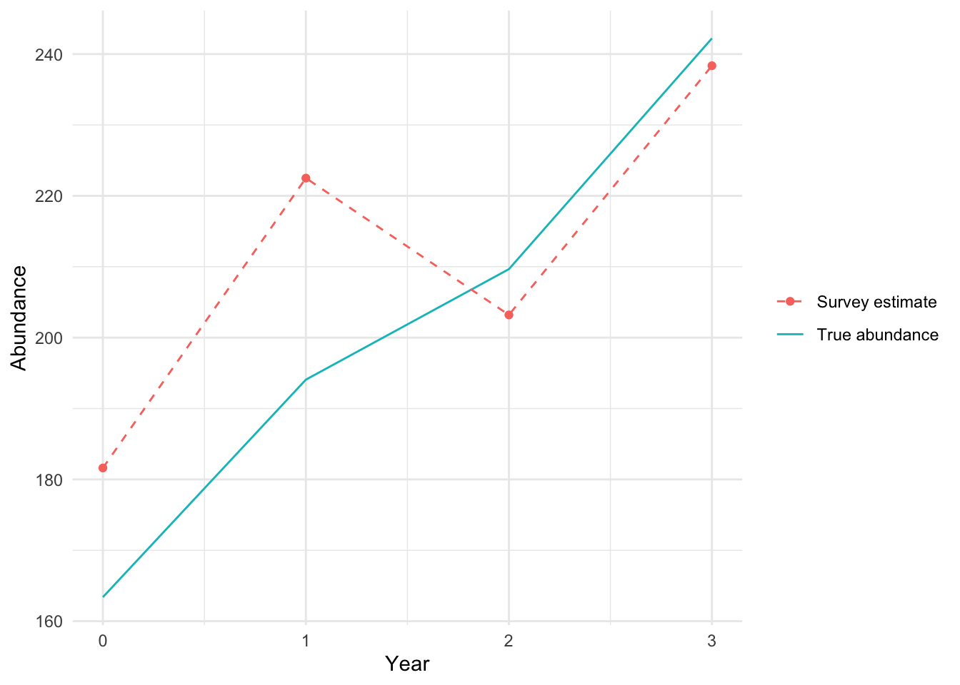
If you mistook the gap between these two lines for as population change, you’d be confounding observation error with process uncertainty.
Peterman, Randall M. 2004. “Possible Solutions to Some Challenges Facing Fisheries Scientists and Managers.” ICES Journal of Marine Science 61 (8): 1331–43. https://doi.org/10.1016/j.icesjms.2004.08.017.
Regan, Helen M., Mark Colyvan, and Mark A. Burgman. 2002. “A Taxonomy and Treatment of Uncertainty for Ecology and Conservation Biology.” Ecological Applications 12 (2): 618–28. https://doi.org/10.1890/1051-0761(2002)012[0618:ATATOU]2.0.CO;2.