How to digitise graphs using R
I recent had reason to digitise some graphs from published papers. You could buy a program to help you do this, but it is actually also possible with R. Here is how to do it.
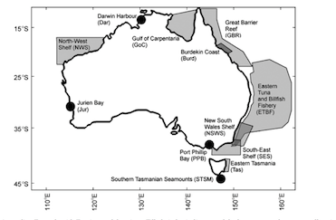
First, take your graph, for instance, here I have taken a screen shot of a map from a paper on ecosystem modelling in Australia. I want to know the coordinates of each of the models plotted on the map. Just the centre point will do for now. You could extract the edges of all the polygons using this method too, but it would be tedious.
Then get and load in the PNG and raster packages, which will allow us to load the image file and plot it in R:
library(png)
library(raster)
pic <- as.raster(readPNG('sole.png'))
Now plot the image on a graph that scales (0,1), so we know where everything has been plotted.
plot(c(0,1), c(0,1))
rasterImage(pic, xleft = 0, xright = 1,
    ybottom = 0, ytop = 1, interpolate = F)
We can use abline() to add some grids to make picking points easier in the following step:
abline(h = seq(0, 1, by = 0.1))
abline(v = seq(0, 1, by = 0.1))
Now use locator() to locate the corners on your imported graph:
xycorners <- locator(2)
xycorners <- cbind(xycorners$x, xycorners$y)
Now enter the values of the corners. For instance, here I used locator to find the bottom left corner (110E by 45 S) and the top right (160E by 15S).
xycvals <- matrix(c(110, 160, -45, -15),
    nrow = 2, byrow = F)
Now we use locator to make twelve clicks (there are twelve models) on each of the locations of the models:
xypts <- locator(12)
xypts3 <- cbind(xypts$x, xypts$y)
Our xypts3 locations are in the (0,1) scale, so then convert these coordinates to the actual coordinates using the locations of the known corners. Here is the conversion for the x-coordinates:
xrise <- xycvals[2,1] - xycvals[1,1]
xrun <- xycorners[2,1] - xycorners[1,1]
xa <- xrise/xrun
xb <- xycvals[1,1] - (xa * xycorners[1,1])
xvals <- xypts3[,1] * xa + xb
Here is the conversion for the y-coordinates:
yrise <- xycvals[2,2] - xycvals[1,2]
yrun <- xycorners[2,2] - xycorners[1,2]
ya <- yrise/yrun
yb <- xycvals[2,2]-(ya * xycorners[2,2])
yvals <- (xypts3[,2] * ya) + yb
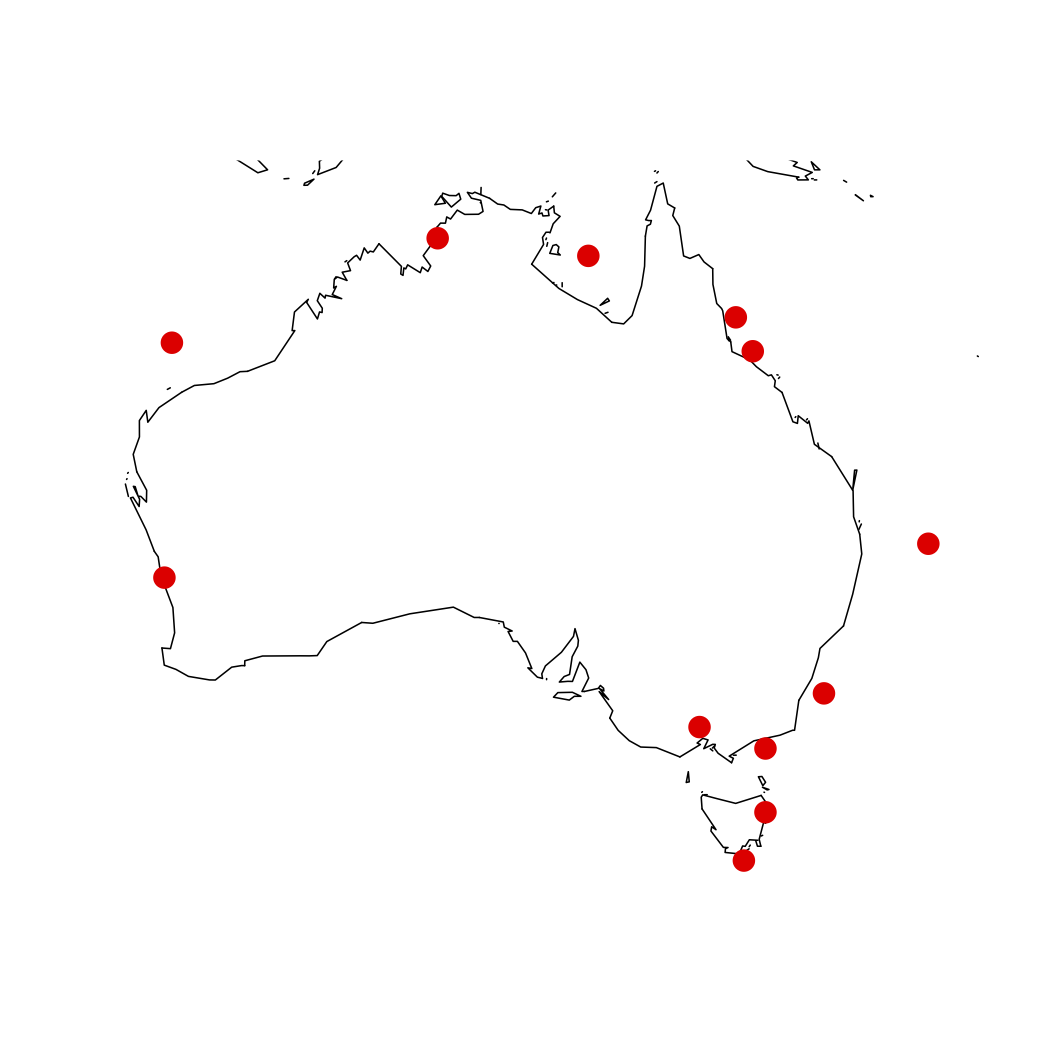
Now we have our true coordinates stored in xvals and yvals. We can replot to check them or save them as a csv for later use. Here we will use the maps library, so we can quickly plot our points back to a map of Australia:
library(maps)
map(database = 'world', xlim = c(110, 160),
   ylim = c(-45, -10))
points(xvals, yvals, pch = 16, col ='red')
write.csv(cbind(xvals, yvals),
   'ecopath-models.csv', row.names = F)
Here is our new map: