Make your R simulation models 20 times faster
R can be frustratingly slow if you use its loops. However, you can speed
it up significantly (e.g. 20 times!) using the Rcpp package. That
could turn a day long simulation into an hour long simulation.
I had heard years ago about the Rcpp package. Rcpp lets you write
and use C ++ functions in R. However, I had never bothered to learn how
to write C ++. Instead if my simulation model got too slow, I just
redefined the problem (e.g. by using smaller spatial domain) so I could
continue with R.

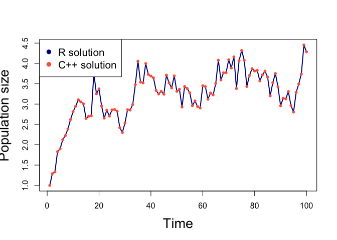
Output of one of the population model runs showing solutions from an R function and an Rcpp function. The C++ version gives an identical results and was up to 20 times faster.
I persisted with R, rather than use another language, because of its powerful graphics and the convenience of using a functional language like R to perform sensitivity analyses. More on this later.
The other day I was browsing Wickhams Advanced R book and realised it is actually pretty easy to write basic C++ loops.
Then I wondered if it would still be faster if you had to make repeated
calls to the same C++ function, for instance if you wanted to run a
sensitivity analysis, varying some model parameters. I like to use R for
this task because the purrr package makes it incredibly easy to run
arbitrary combinations of parameters through a function. Then it is
straightforward to summarize and plot the results with ggplot2.
Turns out you can get a massive improvement, even for repeated calls to the same function. Here is a test.
A population model in R
First up, let’s write a simple model for simulating population size over
time, according to the logistic function. The below function just takes
your standard r (intrinsic population growth) and k (carrying
capacity) parameters and simulates population size starting at yinit
over t years.
Further, to I have included a stochastic process, whose variation is
controlled by thetasd, to illustrate Rcpp random number generator.
logmodr <- function(t, yinit, r, k, thetasd){
    y <- numeric(t)
    y[1] <- yinit
    theta <- rnorm(t, 0, thetasd)
    for(i in 2:t){
        y[i] <- y[i-1]*(r - r*(y[i-1]/k)) * exp(theta[i])
    }
    return(y)
}
Note that I also ran these models without the stochastic component. The speedup was even greater when you compared C++ to R without the stochastic step (about 20 times).
A population model in C++
Now let’s write the equivalent C++ function. You will need to install
the Rcpp package. Note that it has some other software dependencies,
so I recommend you read the guide on
CRAN.
We write the function definition as a string and pass it to
cppFunction from Rcpp:
library(Rcpp)
    cppFunction("NumericVector logmodc(int t, double yinit, double r,
double k, double thetasd){
            NumericVector y(t);
            y[0] = yinit;
      NumericVector theta = rnorm(t, 0, thetasd);
            for (int i = 1; i < t; ++i){
                y[i] = y[i-1]*(r - r*(y[i-1] / k)) * exp(theta[i]);
                }
            return y;
    }
    ")
Hopefully you can understand this, even if you are not familiar with C++. The syntax is reasonably similar to R. If you learned to program in R you may notice a few discrepencies.
First, C++ requires that you specify the type of each variable when its created. You can’t just create new variables without assigning them a type, and you can’t just change the type. This makes C++ more efficient than R, because the computer knows exactly how much memory to allocate a variable and doesn’t have to watch for changes.
Second, notice I start the iterator at time-step 1, whereas in the R
code we started at time-step 2. In C++ vectors are indexed starting at
0.
Finally, don’t forget to end lines with ; (you can use ; to end
lines in R, but it is not essential).
Running a single simulation
First up, we need to define the model parameters:
t <- 100
yinit <- 1
k <- 20
thetasd <- 0.1
r <- 0.2
Now we can run our model. I am just going to plug the models straight
into microbenchmark, so I can compare their times.
library(microbenchmark)
mb1 <- microbenchmark(
    logmodc(t, yinit, 1.4, k, thetasd),
    logmodr(t, yinit, 1.4, k, thetasd)
)
mb1

## Unit: microseconds
##                                expr     min       lq      mean   median
##  logmodc(t, yinit, 1.4, k, thetasd)  10.051  11.1100  12.70373  11.7415
##  logmodr(t, yinit, 1.4, k, thetasd) 179.053 198.8315 251.48889 224.3450
##        uq      max neval cld
##   12.8825   67.801   100  a
##  296.1400 1098.436   100   b
So the C++ version is 19 times faster.
Running multiple simulations
So C++ is faster for a single call to a function (that contains a loop).
No surprises there. What if we want to make repeated calls to the same
function, is C++ still faster than R? We might want to make repeated
calls if we want to run different values of r through our model to do
a sensitivty analysis.
We could increase the scope of the C++ code to include a loop over
different values of r. However, then we would lose some of the
convenience of R, which is good at manipulating data. We also wouldn’t
be able to use purrr package to make sensitivity analysis easy.
First, up let’s create a sequence of r values:
rseq <- seq(1.1, 2.2, length.out = 10)
Now we can run our two models. I will use purrr::map (the :: just
means map is in the package purrr and avoids another call to
library()). We will also use set.seed() to make sure both algorithms
generate the same series of random numbers, that way we can check
whether the results are identical.
set.seed(42)
yc <- purrr::map(rseq, ~logmodc(t, yinit, .x, k, thetasd))
set.seed(42)
yr <- purrr::map(rseq, ~logmodr(t, yinit, .x, k, thetasd))
map iteratively steps through rseq replacing the .x in the
function call with each value of r in turn. Note that we also have to
turn the function call into a formula (with ~) to iterate in this way.
map returns a list, where each element is a time-series of population
sizes for a given value of r.
Let’s plot the result, for the second value of r:
plot(yr[[2]], type = "l", col = "DarkBlue", lwd = 2)
points(yc[[2]], pch = 16, col = "Tomato", cex = 0.8)
legend('topleft', legend = c("R solution","C solution"),
       pch = 16, col = c("DarkBlue", "Tomato"))

They look identical, excellent.
Now, let’s compare the time. Remember I had wondered whether repeated calls to a C++ function might lose some of the performance gain:
mb2 <- microbenchmark(
    purrr::map(rseq, ~logmodc(t, yinit, .x, k, thetasd)),
    purrr::map(rseq, ~logmodr(t, yinit, .x, k, thetasd))
)
mb2

## Unit: microseconds
##                                                  expr      min        lq
##  purrr::map(rseq, ~logmodc(t, yinit, .x, k, thetasd))  151.421  166.4165
##  purrr::map(rseq, ~logmodr(t, yinit, .x, k, thetasd)) 1890.549 2047.6310
##       mean    median       uq      max neval cld
##   199.9101  179.5795  221.885  371.192   100  a
##  2543.3459 2233.7455 2534.350 9173.440   100   b
Turns out we still gain a 12 times improvement when using C++.
I don’t believe I have been wasting so many hours waiting for simulations to run all these years. Learning a bit of C++ is well worth the investment.