Fast functions with pipes
Pipes are becoming popular R syntax, because they help make code more readable and can speed up coding. You can even use pipes to create functions. This is handy if you want to repeat a piped process for several different datasets.
Trivial example
Let’s start with a trivial example. You can access pipes through the
tidyverse or the original magrittr package.
We’ll create a function that plots a data series in rank order:
library(magrittr)
rank_plot <- . %>%
  sort() %>%
  plot()
So to create a function out of a pipe we just start the pipe with the
..
Now rank_plot has no data, but is rather what is called a ‘functional
sequence’. Type rank_plot in your console to see this.
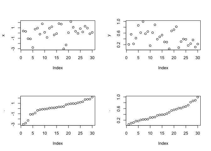
Let’s use it to plot two randomly generated variables:
set.seed(2020)

x <- rnorm(30)
y <- runif(30)

par(mfrow = c(2,2))
plot(x) #x data in original order
plot(y) # y data in original order
rank_plot(x) #rank ordered data
rank_plot(y)
Maps
Let’s true a slightly more sophisticated example, a map.
We’ll use tmap to make the maps.
First access some data. Here I’ve picked a couple of random mushroom species that have data on the Queensland Government’s Wetland Info page. The data-tables record (rather out-of-date) observations of the species and the sites where they were recorded. This data is just for the area around Brisbane where I live:
amanita <- read.csv(url("http://apps.des.qld.gov.au/species/?op=getsurveysbyspecies&taxonid=25531&f=csv"))
psilocybe <- read.csv(url("http://apps.des.qld.gov.au/species/?op=getsurveysbyspecies&taxonid=28689&f=csv"))
names(psilocybe)

##  [1] "ID"                  "Longitude"           "Latitude"
##  [4] "TaxonID"             "ScientificName"      "SiteVisitID"
##  [7] "StartDate"           "EndDate"             "SiteID"
## [10] "SiteCode"            "LocalityDetails"     "LocationPrecision"
## [13] "ProjectID"           "ProjectName"         "OrganisationID"
## [16] "OrganisationName"    "OrganisationAcronym"
I’ve wrapped the web addresses in the url() function as they are web
datasources.
Now to the maps. First, let’s make a function out of a tmap call:
library(tmap)
library(sf)

## Linking to GEOS 3.8.1, GDAL 3.1.1, PROJ 6.3.1

mymap <- . %>%
  st_as_sf(coords = c("Longitude", "Latitude")) %>%
  {tm_shape(.) +
  tm_markers()}
If you want the map to be interactive, do this next:
tmap_mode("view")
tmap_options(basemaps = c(Canvas = "Esri.WorldTopoMap"))
The function first converts the csv to a spatial points (st_points)
object, then maps that data. Note I had to wrap the map in {} to
include it at the end of the pipe.
Now we can use it to map any of our dataframes. For instance:
# mymap(amanita)
mymap(psilocybe)
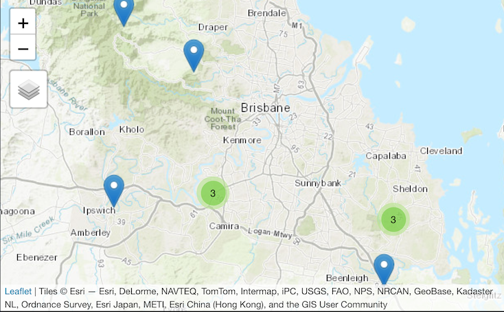
(This is a screen shot, but if you do this yourself it will be interactive)
Conclusion
So pipes are also handy for creating quick functions. This could also be
very useful in situations where we pipe a series of dplyr functions to
wrangle a dataset. They could be combined with loops, apply or
pmap::map to repeat the call for different dataset.
One thing that I find challenging with %>% is debugging is very hard. So a word
of warning, keep your pipes short and simple so they are easy to debug
(or use one of the specialist pipe debugging packages).
Pipes will likely be included in base R soon, and the R Core team are promising to make them more debuggable.
Enjoy.