Comparison of terra and stars packages
The other day I wrote a comparison of raster and terra packages. The other newish raster package on the block is stars. So I go through the same code here.
If you are starting out with stars, read their manual first.
But first some key differences.
stars is set-up to work with spatio-temporal arrays (terra also has better capacity to work with multilayer rasters than raster did). stars deals with more complex data types than either raster or terra, for instance, stars can handle rotated grids.
stars works will with sf, and many sf functions have methods for
stars objects (like st_bbox and st_transform). In contrast, my
current experience of trying to use terra and sf is a bit more
awkward. I had to do lots of class conversions of terra objects to
sf objects and back again.
stars isn’t as well documented as raster or terra. Some colleagues
told me they’ve had unresolvable issues with stars and reverted to
raster. I don’t know the details though.
There is a ‘babel’ for stars to raster function names though.
Data reading and plotting in stars
Data input and plots are quite similar to sf:
library(stars)
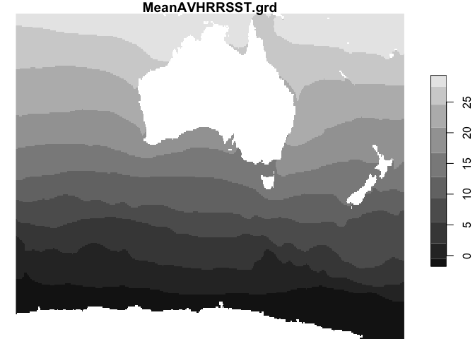
r <- read_stars("data-for-course/spatial-data/MeanAVHRRSST.grd")
plot(r)

st_bbox(r)

##   xmin   ymin   xmax   ymax
##  82.50 -72.25 181.25  -9.75
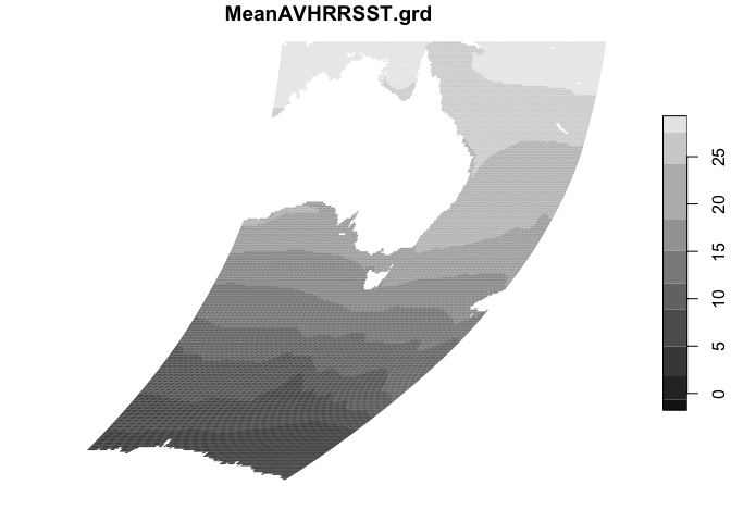
Now let’s crop and reproject it, it looks almost identical to
reprojecting a polygon in sf:
#create an extent object
ext2 <- st_bbox(r)

#constrain it in x direction
ext2[1] <- 120
ext2[3] <- 170

r2 <- st_crop(r, ext2)

r3 <- st_transform(r2, "+proj=robin +lon_0=0 +x_0=0 +y_0=0 +ellps=WGS84 +datum=WGS84 +units=m +no_defs +towgs84=0,0,0")

plot(r3)

How do terra, raster and stars compare for speed?
Let’s compare the three packages for speed at projecting data, an often time-consuming task.
library(microbenchmark)

r_terra <- terra::rast("data-for-course/spatial-data/MeanAVHRRSST.grd")
r_raster <- raster::raster("data-for-course/spatial-data/MeanAVHRRSST.grd")

robin_proj <- "+proj=robin +lon_0=0 +x_0=0 +y_0=0 +ellps=WGS84 +datum=WGS84 +units=m +no_defs +towgs84=0,0,0"

tout <- microbenchmark(
raster::projectRaster(r_raster, crs=robin_proj),
terra::project(r_terra, robin_proj),
st_transform(r, crs = robin_proj),
times = 10
)
tout

## Unit: milliseconds
##                                               expr       min        lq
##  raster::projectRaster(r_raster, crs = robin_proj) 330.49234 348.60983
##                terra::project(r_terra, robin_proj)  66.47145  67.78466
##                  st_transform(r, crs = robin_proj)  19.03904  19.91101
##       mean    median        uq       max neval
##  506.93616 505.29937 521.27790 874.32388    10
##   69.90088  68.87271  69.09739  80.66674    10
##   23.38595  20.64656  22.88241  42.57163    10
So terra was about 8.5 times faster than raster and stars was
about 3 times faster than terra (so about 26 times faster than
raster).
Will stars be compatible with other packages I use?
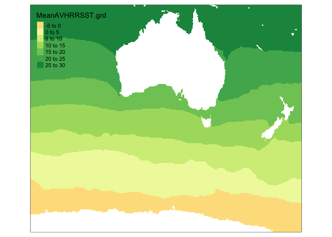
The answer here obviously depends on what packages you want to use. A key one for me is tmap for mapping:
library(tmap)
tm_shape(r) +
  tm_raster()
 Apparently you can
 coerce stars objects into raster objects, but I
couldn’t figure out easily how to do that (with the 10 minutes I had to
find out).
Summary
Its a confusing world of raster packages now, with raster, terra and stars all viable options. A decision about your ‘go to’ package needs more exploration than my brief blog and will depend on what types of operations you are doing.
The real test will come when analyzing large and complex datasets. The comparison I’ve made here is very shallow, it doesn’t explore the full functionality of terra or stars, which is much deeper than raster. So I’m interested to hear from folk how they go with more sophisticated applications.